Quantopian 讲义翻译 1:打造更好的 Beta
本文是《Maeiee 量化学习路线图之 Quantopian》中,对《Building a Better Beta》一文的翻译。
今天我们宣布发布 SimpleBeta,这是一个新的 Pipeline API,使你能够轻松有效地计算交易范围内所有股票的市场 beta。
在本文中,我们介绍了市场 beta 的概念,并展示了 SimpleBeta 是如何改进 Pipeline 中的已有工具来计算 beta。
大纲:
- 介绍市场 beta,并解释为什么我们在交易算法的背景下会关心它。
- 展示我们以前如何使用 RollingLinearRegressionOfReturns 来计算大量资产的市场 beta。
- 展示我们如何从第一原理出发,以 CustomFactor 的形式建立一个更快的 beta 实现。
- 介绍新的 SimpleBeta 内置因子,它比 RollingLinearRegressionOfReturns 快130倍以上,并且可以处理丢失的输入数据。
什么是 beta,我们为什么要关心它?
当股票价格变动时,它们往往与整个市场的变动同步。然而,并不是所有的股票都同样表现出这种趋势:一些股票在历史上对市场的运动有的很敏感,有的不太敏感。
衡量一只股票在多大程度上倾向于与市场的其他部分一起移动的一个简单方法,是在市场的回报和有关股票的回报之间进行线性回归。这种回归的斜率给了我们一种衡量方式,来衡量资产的回报率受整个市场回报率影响的力度。
由于线性回归方程通常被写成:
$\displaystyle{ \begin{equation} \begin{split} Y \sim \alpha + \beta X \end{split} \end{equation} }$
(读作:Y 的分布为 α 加βX)我们通常把资产收益和市场收益之间的回归线的斜率称为资产的 "市场 beta"。
使用 scipy 计算 beta
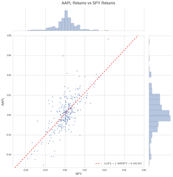
让我们看看我们如何计算 AAPL 的 beta 值。一个简单的方法是使用 scipy.stats.linregress 对每日回报率进行线性回归。在实践中,我们经常使用像 SPY 这样的大盘 ETF 的价格作为 "市场 "回报的代理。
from __future__ import print_function

import numpy as np
import pandas as pd
from quantopian.research import returns

START = pd.Timestamp('2010-01-04')
END = pd.Timestamp('2010-12-31')

# Load returns for AAPL (Apple Computer) and SPY (an ETF often used as a proxy for the market).
rets = returns(['AAPL', 'SPY'], START, END)
AAPL, SPY = rets.columns

# Show the first 5 rows.
rets.head()
输出:
| Equity(24 [AAPL]) | Equity(8554 [SPY]) | Equity(8554 [SPY]) |
|---|---|---|
| 2010-01-04 00:00:00+00:00 | 0.015841 | 0.016872 |
| 2010-01-05 00:00:00+00:00 | 0.000934 | 0.002735 |
| 2010-01-06 00:00:00+00:00 | -0.016046 | 0.000960 |
| 2010-01-07 00:00:00+00:00 | -0.001707 | 0.004052 |
| 2010-01-08 00:00:00+00:00 | 0.006221 | 0.003232 |
linregress 返回一个包含斜率、截距和其他一些关于回归的有用统计数据的 namedtuple。
from scipy.stats import linregress
linregress(x=rets[SPY].values, y=rets[AAPL].values)
输出:
LinregressResult(slope=1.0688251632444647, intercept=0.0011645457531190501, rvalue=0.71261796119874299, pvalue=2.3069534088276338e-40, stderr=0.066548758680318718)
这个回归告诉我们,2010 年,AAPL 对 SPY 的 beta 值略高于1.0。这不应该是非常令人惊讶的。苹果是这样一家大公司,它的回报占了整个市场回报的很大一部分。
我们可以用 matplotlib 和 seaborn 将回归的结果可视化。
import matplotlib.pyplot as plt
import seaborn as sns

def regression_plot(data, size=11, legend_position='lower right'):
    """Calculate and plot a linear regression between two columns of data.

    Parameters
    ----------
    data : pd.DataFrame
        DataFrame with two columns to be regressed and plotted.
        The first column of the frame will be plotted on the y-axis.
        The secont column of the frame will be plotted on the x-axis.
    figsize : tuple, optional
        Size of the resulting figure in (x_inches, y_inches)
    legend_position : string
        Location on the plot for the legend.

    Returns
    -------
    ax : matplotlib.axes.Axes
        Axes containing the scatterplot and regression line.
    """
    ylabel, xlabel = data.columns

    # Draw scatterplot with marginals using seaborn.
    grid = sns.jointplot(x=data[xlabel], y=data[ylabel],
                         size=size, joint_kws={'alpha': 0.6, 'linewidth': 0})

    # The plot generated by seaborn is composed of three matplotlib.Axes objects.
    # The scatter plot is drawn on ax_joint. Draw a regression line on top of the scatter plot.
    axes = grid.ax_joint
    draw_regression_line(Y=data[ylabel], X=data[xlabel], ax=axes)

    # Set X and Y Axis Bounds
    min_ = data.values.min() * 1.05  # Leave a margin at the edge of the figure.
    max_ = data.values.max() * 1.05
    axes.set_ylim(min_, max_)
    axes.set_xlim(min_, max_)

    # Draw legend.
    axes.legend(fontsize=13, loc=legend_position)

    # Set title on the overall figure.
    grid.fig.suptitle(
        '{} Returns vs {} Returns'.format(ylabel.symbol, xlabel.symbol),
        size=18,
        y=1.02
    )

    # Set axis label sizes.
    axes.set_ylabel(ylabel.symbol, size=15)
    axes.set_xlabel(xlabel.symbol, size=15)

    return axes

def draw_regression_line(Y, X, ax=None):
    """Calculate and plot a linear regression line.

    Parameters
    ----------
    Y : np.array or pd.Series
        Y values for the regression.
    X : np.array or pd.Series
        X values for the regression.
    ax : matplotlib.Axes, optional
        Axes on which to draw the line.
        If not passed, default is ``matplotlib.pyplot.gca()``.
    """
    if ax is None:
        ax = plt.gca()

    result = linregress(x=X, y=Y)
    slope = result.slope
    intercept = result.intercept

    x_endpoints = np.array([X.min(), X.max()]) * 2
    y_endpoints = intercept + slope * x_endpoints

    # Format a regression equation in LaTeX.
    plot_label = "${} = {:.4g}{} {} {:.4g}$".format(
        r'\mathrm{' + Y.name.symbol + '}',
        slope,
        r'\mathrm{' + X.name.symbol + '}',
        '+' if intercept > 0 else '-',
        abs(intercept),
    )

    ax.plot(x_endpoints, y_endpoints, label=plot_label, linestyle='--', color='red', linewidth=2)
    return ax
regression_plot(rets);
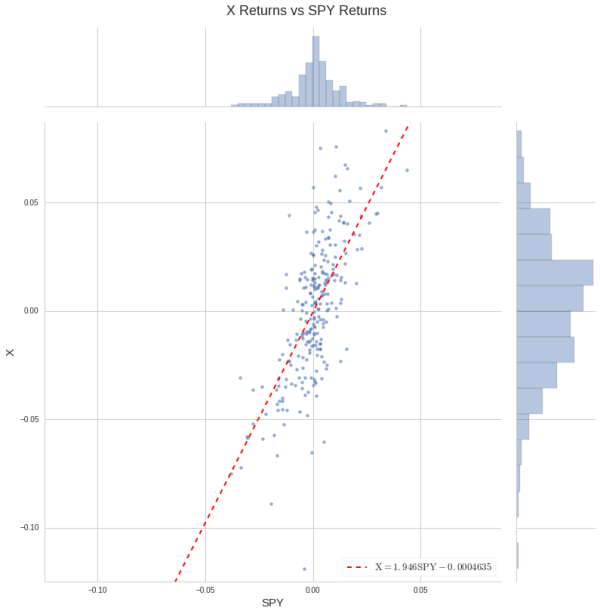
大多数股票至少显示出一些历史趋势,随着整体市场移动,但不同的股票在不同时期会显示出不同的敏感性。
例如,联合钢铁公司(X),在历史上对市场比大多数股票更敏感。
X = returns('X', START, END)
linregress(x=rets[SPY].values, y=X.values)
LinregressResult(slope=1.9457293114742904, intercept=-0.00046346369353660131, rvalue=0.69485844565998056, pvalue=1.156540205721078e-37, stderr=0.12736012290975701)
regression_plot(returns(['X', 'SPY'], START, END));
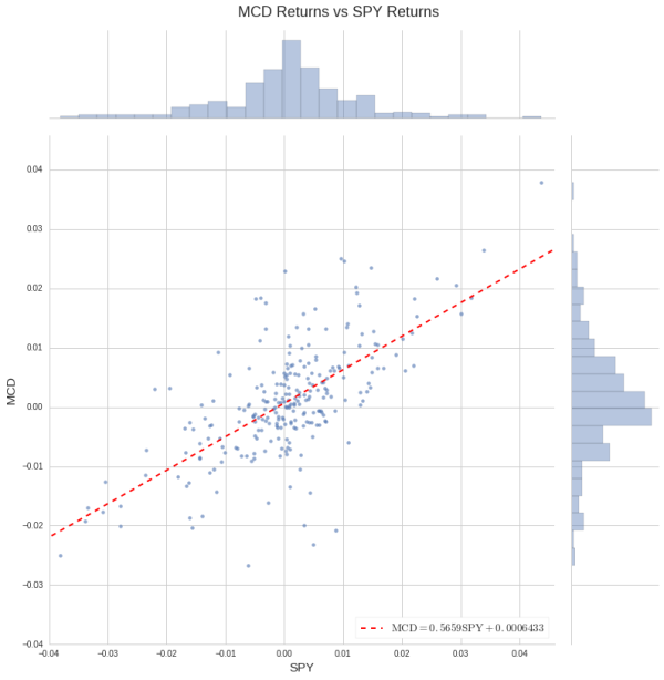
MCD = returns('MCD', START, END)
linregress(x=rets[SPY].values, y=MCD.values)
LinregressResult(slope=0.56593257597506752, intercept=0.00064333935781934375, rvalue=0.66624361151729328, pvalue=1.0538531257566855e-33, stderr=0.040063203555931105)
regression_plot(returns(['MCD', 'SPY'], START, END));
使用 Pipeline 计算所有股票的 Beta
在一个交易大量资产的算法中,了解每只股票对市场的历史 beta 值往往是有用的。例如,试图控制算法的市场 beta 值的一种方法是使算法的头寸的 beta 加权风险接近于零。
长期以来,Pipeline API 提供了一个名为 RollingLinearRegressionOfReturns 的内置因子,可以用来计算 Quantopian 数据库中所有资产的简单线性回归。
RollingLinearRegressionOfReturns 的实现基本上可以归结为这样的内容:
from quantopian.pipeline.factors import CustomFactor, DailyReturns

class MyRollingLinearRegressionOfReturns(CustomFactor):
    outputs = ['alpha', 'beta', 'r_value', 'p_value', 'stderr']
    inputs = [DailyReturns(), DailyReturns()[symbols('SPY')]]

    def compute(self, today, assets, out, dependent, independent):
        alpha = out.alpha
        beta = out.beta
        r_value = out.r_value
        p_value = out.p_value
        stderr = out.stderr

        def regress(y, x):
            regr_results = linregress(y=y, x=x)
            alpha[i] = regr_results.intercept
            beta[i] = regr_results.slope
            r_value[i] = regr_results.rvalue
            p_value[i] = regr_results.pvalue
            stderr[i] = regr_results.stderr

        for i in range(len(out)):
            regress(y=dependent[:, i].ravel(), x=independent.ravel())
(截至本文写作时,RollingLinearRegressionOfReturns 的完整来源可以在 Zipline 这里找到)。
该类使用 CustomFactor 的多重输出功能,每天同时输出 scipy.stats.linregress 计算的所有数值。
我们可以用它来计算 Quantopian 数据库中每个资产的滚动 beta,就像这样:
from quantopian.pipeline import Pipeline
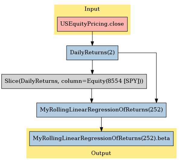
regression = MyRollingLinearRegressionOfReturns(window_length=252) # two year lookback
pipeline = Pipeline({'beta': regression.beta})
这个 pipeline 的计算图看起来像这样:
pipeline.show_graph('png')
from quantopian.research import run_pipeline

betas = run_pipeline(pipeline, END, END)
betas.head()
| beta | ||
|---|---|---|
| 2010-12-31 00:00:00+00:00 | Equity(2 [ARNC]) | 1.556766 |
| Equity(21 [AAME]) | NaN | |
| Equity(24 [AAPL]) | 1.067143 | |
| Equity(25 [ARNC_PR]) | NaN | |
| Equity(31 [ABAX]) | 1.188185 |
不幸的是,对于 RollingLinearRegressionOfReturns 来说,每天循环查看每一列输入并每次调用 scipy.stats.linregress 并不是很有效率,尤其是当我们只关心回归的斜率时。
在纯 Python 中对 numpy 数组进行循环是很慢的,而且 linregress 的实现在设计时没有考虑到它会被大量调用,所以它做了一些昂贵的事情,比如每次调用都要定义一个新的 namedtuple 子类。
linregress 还计算截距、P值、R平方值和估计值的标准误差(都是相对昂贵的计算),但如果我们只关心回归的斜率,这些计算就白费了。
我们可以用 RollingLinearRegressionOfReturns 来衡量计算 betas 的大致时间,使用 time.time 和一点小聪明。
import time
def timed(f):
    """Take a function f and return a **new function** that calls f and returns a pair
    containing f's result and how long it took to compute.
    """
    def timed_f(*args, **kwargs):
        start = time.time()
        result = f(*args, **kwargs)
        end = time.time()
        difference = end - start
        return result, difference
    return timed_f
# This cell should take about 45 seconds to execute.

result, duration = timed(run_pipeline)(pipeline, '2009-01-02', '2009-01-02')
print("It took {} seconds to calculate 252-day betas for 1 day:".format(duration))

result, duration = timed(run_pipeline)(pipeline, '2009-01-02', '2009-01-10')
print("It took {} seconds to calculate 252-day betas for 5 trading days:".format(duration))
It took 6.37987399101 seconds to calculate 252-day betas for 1 day:
It took 39.0593450069 seconds to calculate 252-day betas for 5 trading days:
每天 6 秒的时间转化为每个回测年度约 25 分钟,这意味着使用 RollingLinearRegressionOfReturns 计算所有资产的 beta 值的两年回测可能要花一个多小时!
幸运的是,我们可以通过自己把 beta 计算写成向量的 numpy 操作来加速我们的计算。
加速 Beta 计算
让我们回顾一下线性回归的数学原理,看看我们是否能找到一种更快的方法来实现我们的 beta 计算。
计算自变量 X 和因变量 Y 的简单线性回归的斜率,最简单和最常用的方法是使用公式:
$\displaystyle{ \begin{equation} \begin{split} \beta = \frac{Cov * sample(X,Y)}{Cov * sample(X,X)}\end{split} \end{equation} }$
其中 $\displaystyle{ Cov_{sample}(X,Y) }$ 是 X 和 Y 的样本协方差。
我在这里使用的 sample 下标是一点非标准的协方差定义,是对一对随机变量 "一起移动 "程度的统计测量。样本协方差是一种从一组观测值中估计分布的协方差的特殊方式。
有很多巧妙地方法来可靠估计协方差(你可以在Quantopian讲座系列中关于协方差估计的文章中阅读其中一些微妙之处)。然而现在,我们只想专注于重新创建 scipy.stats.linregress 所做的事情,但要更快。
给出从 X 种抽取的一组观测 $\displaystyle{ x_1, x_2,\dots,x_N }$ ,和从 Y 种抽取的一组观测 $\displaystyle{ y_1, y_2,\dots,y_N }$ ,样本的协方差是:
$\displaystyle{ \begin{equation} \begin{split} Cov * sample(X, Y) = \frac{1}{N-1}\sum{*i=1^N(x_i-\bar{X})(y_i-\bar{Y})} \end{split} \end{equation} }$
其中 $\displaystyle{ \bar{X} }$ 是 $\displaystyle{ x_1, x_2,\dots,x_N }$ 的采样均值,$\displaystyle{ \bar{Y} }$ 是 $\displaystyle{ y_1, y_2,\dots,y_N }$ 的采样均值。
上面公式可以按照如下理解:
- 对于每一组观测 (xi, yi),看看 xi 高于或低于所有 x 的平均值的程度,然后用这个值乘以 yi 高于或低于所有 y 的平均值的程度。
- 如果 xi 和 yi 都高于或者低于平均程度,则 $\displaystyle{ (x_i-\bar{X})(y_i-\bar{Y}) }$ 得到一个正值
- 如果 xi 和 yi 位于各自平均程度的对立侧,则 $\displaystyle{ (x_i-\bar{X})(y_i-\bar{Y}) }$ 得到一个负值
- 为了计算样本协方差,我们取所有这些均差乘积的平均值,只不过在计算均值时,我们除以 N-1 而不是 N,以纠正我们同时估计估计均值和协方差所带来的微小偏差。
- 如果在我们的数据中,高于平均水平的 x 样本往往对应于高于平均水平的 y 样本,那么我们最终将对大多数的正值取平均。因此我们将估计出一个正的协方差。
- 如果低于平均水平的 x 样本往往对应于高于平均水平的 y 样本,我们最终会平均化大部分的负值,所以我们会估计一个负的协方差。
- 如果 x 高于其平均值和 y 高于其平均值之间没有任何关系,那么我们最终会对正负值进行混合平均,所以我们最终会得到一个接近零的协方差。
由于我们感兴趣的是测量每种资产的回报如何取决于市场的回报,我们的自变量 X 将是 SPY 的回报,而我们的因变量 Y 将是我们要计算的 beta 值的资产的回报。
为了开始,让我们看看是否可以通过尽可能地复制上面的公式来加速我们的单一股票 beta 计算。
def timeit(f):
    """Take a function f and return a new function that calls 5000 times,
    returning the last result and the average runtime, ignoring the ten
    slowest/fastest calls. This gives a more reliable estimate for fast functions.
    """
    _time=time.time
    def timed_f(*args, **kwargs):
        times = []
        for _ in range(5000):
            start = _time()
            result = f(*args, **kwargs)
            end = _time()
            times.append(end - start)
        # Take the average of the middle three to smooth out variance from cache effects.
        average_time = sum(sorted(times)[10:-10]) / (len(times) - 20)
        return result, average_time
    return timed_f
def beta_v0(spy, asset):
    """Calculate the slope of a linear regression for one asset with SPY.
    """
    asset_residuals = asset - asset.mean()
    spy_residuals = spy - spy.mean()

    covariance = (asset_residuals * spy_residuals).sum() / (len(asset) - 1)
    spy_variance = (spy_residuals ** 2).sum() / (len(asset) - 1)

    return covariance / spy_variance

v0_result, v0_duration = timeit(beta_v0)(rets[SPY].values, rets[AAPL].values)
print("Our AAPL beta is {}. Calculation took {} seconds.".format(v0_result, v0_duration))

scipy_result, scipy_duration = timeit(linregress)(rets[SPY].values, rets[AAPL].values)
print("linregress AAPL beta is {.slope}. Calculation took {} seconds.".format(
    scipy_result, scipy_duration
))
print()
print("Our calculation was {} times faster than linregress.".format(scipy_duration / v0_duration))
Our AAPL beta is 1.06882516324. Calculation took 2.93323313855e-05 seconds.
linregress AAPL beta is 1.06882516324. Calculation took 0.000671482660684 seconds.
Our calculation was 22.8922362788 times faster than linregress.
到目前为止还不错。我们可以准确地重现scipy的结果,而且通过避免我们不需要的额外计算,我们已经得到了显著的速度提升。
我们可以通过注意到我们在用 covariance 和 spy_variance 除以 N-1 来加快我们的执行速度,尽管我们接下来要做的事情是用 covariance 除以 spy_variance。因为除以 N-1 最终会被抵消,所以我们不需要在第一时间去处理它们。
def beta_v1(spy, asset):
    """Calculate the slope of a linear regression for one asset with SPY.
    """
    asset_residuals = asset - asset.mean()
    spy_residuals = spy - spy.mean()

    # These variable names aren't really correct anymore since we're
    # taking a sum instead of a mean, but I couldn't think of better names.
    covariance = (asset_residuals * spy_residuals).sum()  # Not dividing here anymore.
    spy_variance = (spy_residuals ** 2).sum()             # Not dividing here anymore.

    return covariance / spy_variance

v1_result, v1_duration = timeit(beta_v1)(rets[SPY].values, rets[AAPL].values)
print("Our AAPL beta is still {}. Calculation took {} seconds.".format(v1_result, v1_duration))
print("Our calculation was {} times faster than linregress.".format(scipy_duration / v1_duration))
Our AAPL beta is still 1.06882516324. Calculation took 2.81569469406e-05 seconds.
Our calculation was 23.8478504825 times faster than linregress.
一旦我们有了一个高效的单一资产的实现,我们就可以对它进行调整,利用多维数组和 numpy 广播对多个资产进行有效的矢量回归。
def vectorized_beta(spy, assets):
    """Calculate beta between every column of ``assets`` and ``spy``.

    Parameters
    ----------
    spy : np.array
        An (n x 1) array of returns for SPY.
    assets : np.array
        An (n x m) array of returns for m assets.
    """
    assert len(spy.shape) == 2 and spy.shape[1] == 1, "Expected a column vector for spy."

    asset_residuals = assets - assets.mean(axis=0)
    spy_residuals = spy - spy.mean()

    covariances = (asset_residuals * spy_residuals).sum(axis=0)
    spy_variance = (spy_residuals ** 2).sum()
    return covariances / spy_variance
让我们看看我们的矢量贝塔如何处理计算 QTradableStocksUS 中每项资产的 beta。
from quantopian.pipeline.experimental import QTradableStocksUS

def get_qtradable_for(day):
    """Get the QTradableStocksUS for a single day.
    """
    pipe = Pipeline({}, screen=QTradableStocksUS())
    result = run_pipeline(pipe, day, day)
    return result.index.get_level_values(1)

universe = get_qtradable_for(END)
print(universe[:5])
Index([ Equity(2 [ARNC]), Equity(24 [AAPL]), Equity(41 [ARCB]),
        Equity(52 [ABM]),  Equity(62 [ABT])],
      dtype='object')
all_returns = returns(universe, START, END).dropna(how='any', axis=1)
all_returns.head()
| Equity(2 [ARNC]) | Equity(24 [AAPL]) | Equity(41 [ARCB]) | Equity(52 [ABM]) | Equity(62 [ABT]) | Equity(64 [ABX]) | Equity(67 [ADSK]) | Equity(76 [TAP]) | Equity(88 [ACI]) | Equity(107 [ACV]) | ... | Equity(38936 [DG]) | Equity(38944 [RUE]) | Equity(38965 [FTNT]) | Equity(38971 [CLD]) | Equity(38989 [AOL]) | Equity(39047 [PEB]) | Equity(39053 [CIT]) | Equity(39073 [CIE]) | Equity(39079 [KRA]) | Equity(39111 [PPC]) | |
|---|---|---|---|---|---|---|---|---|---|---|---|---|---|---|---|---|---|---|---|---|---|
| 2010-01-04 00:00:00+00:00 | 0.032252 | 0.015841 | -0.030593 | 0.029578 | 0.010002 | 0.024628 | 0.010232 | 0.018168 | 0.055314 | 0.020497 | ... | 0.026304 | -0.017475 | 0.024474 | 0.019231 | 0.023555 | -0.030863 | 0.026792 | 0.037037 | 0.015453 | 0.002247 |
| 2010-01-05 00:00:00+00:00 | -0.031244 | 0.000934 | -0.003839 | -0.006422 | -0.009163 | 0.012631 | -0.015193 | -0.013494 | 0.045354 | -0.009028 | ... | 0.009557 | 0.004356 | 0.019444 | 0.017520 | 0.030962 | 0.018231 | 0.049718 | 0.053922 | 0.044928 | -0.035874 |
| 2010-01-06 00:00:00+00:00 | 0.050914 | -0.016046 | -0.007036 | 0.001944 | 0.006472 | 0.021761 | 0.002373 | -0.001334 | 0.062531 | -0.004743 | ... | 0.016351 | 0.068666 | 0.059946 | 0.070861 | 0.006494 | 0.000463 | 0.065166 | -0.011296 | 0.012483 | 0.029070 |
| 2010-01-07 00:00:00+00:00 | -0.020678 | -0.001707 | -0.014528 | 0.010428 | 0.008104 | -0.014118 | 0.005525 | -0.015010 | 0.026052 | 0.006445 | ... | 0.003810 | 0.035847 | -0.002057 | 0.012369 | -0.006855 | -0.017943 | 0.000315 | 0.016801 | 0.000000 | -0.018079 |
| 2010-01-08 00:00:00+00:00 | 0.024705 | 0.006221 | 0.016513 | -0.000432 | 0.004567 | 0.005811 | 0.030534 | -0.002459 | 0.002243 | -0.018872 | ... | 0.009701 | 0.061051 | 0.034003 | 0.013439 | 0.042631 | -0.011207 | 0.016709 | 0.019828 | 0.020548 | -0.010357 |
5 rows × 1755 columns
# Convert 1D array of spy returns into an N x 1 2D array.
SPY_column = rets[SPY].values[:, np.newaxis]
betas, duration = timed(vectorized_beta)(SPY_column, all_returns.values)

print("AAPL beta is still", betas[all_returns.columns.get_loc(AAPL)])
print("It took {} seconds to calculate betas for {} stocks.".format(duration, len(betas)))
AAPL beta is still 1.06882516324
It took 0.00327587127686 seconds to calculate betas for 1755 stocks.
现在我们开始有进展了! 如果我们每个交易日花 0.002 秒计算 beta,那么这意味着我们每个回测年只花了大约半秒计算 beta。
0.002 * 252
0.504 让我们看看如何将我们的 vectorized_beta 函数插入 CustomFactor中。
SPY_asset = symbols('SPY')

daily_returns = DailyReturns()

class MyBeta(CustomFactor):
    # Get daily returns for every asset in existence, plus the daily returns for just SPY
    # as a column vector.
    inputs = [daily_returns, daily_returns[SPY_asset]]
    # Set a default window length of 2 years.
    window_length = 252

    def compute(self, today, assets, out, all_returns, spy_returns):
        out[:] = vectorized_beta(spy_returns, all_returns)
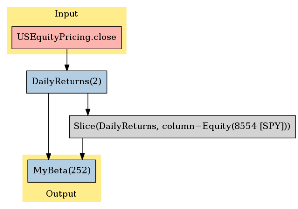
my_beta_pipeline = Pipeline({'beta': MyBeta()})
my_beta_pipeline.show_graph('png')
my_betas, duration = timed(run_pipeline)(my_beta_pipeline, END, END)
print("AAPL's beta is still", my_betas.xs(AAPL, level=1).values[0, 0])
print("It took {} seconds to calculate 252-day betas for 1 day:".format(duration))
AAPL 的 beta 值仍然是1.06714326974
计算 1 天的 252日 beta 值需要 0.623263835907 秒。
我们从花 6 秒来计算一天的 beta,到现在只花了半秒多的时间!
实际上,我们做得比这些数字看起来还要好:这半秒中的大部分时间是用来加载定价数据的,而不是计算 beta,所以如果我们运行的时间更长,我们的扩展性会更好。
from zipline.utils.calendars import get_calendar
NYSE = get_calendar('NYSE')
my_beta_result, duration = timed(run_pipeline)(my_beta_pipeline, END, END + (5 * NYSE.day))
print("It took {} seconds to calculate 252-day betas for 5 trading days:".format(duration))

my_beta_result, duration = timed(run_pipeline)(my_beta_pipeline, END, END + (40 * NYSE.day))
print("It took {} seconds to calculate 252-day betas for two months:".format(duration))

my_beta_result, duration = timed(run_pipeline)(my_beta_pipeline, END, END + (252 * NYSE.day))
print("It took {} seconds to calculate 252-day betas for a year:".format(duration))
It took 0.695220947266 seconds to calculate 252-day betas for 5 trading days:
It took 1.36936211586 seconds to calculate 252-day betas for two months:
It took 5.96089887619 seconds to calculate 252-day betas for a year:
我们更新的 MyBeta factor,在计算全年 beta 时,过去要花上一天,而现在几秒钟搞定。
超过 250 倍的优化!
SimpleBeta 内置 Factor
我们仍有一些方法可以提高我们的 MyBeta Factor:
- 我们可以增加对 SPY 以外的资产进行回归的支持(例如,对行业ETF)。
- 我们可以增加对处理缺失数据的更好支持(例如,如果我们正在计算1年的 beta 系数,我们可能仍然希望使用我们拥有的数据为 6 个月前上市的股票计算一个 "尽力而为 "的 beta。)
- 我们可以通过一些技巧来加快性能,尽可能避免进行不必要的复制。
幸运的是,我们不需要在这里实现所有这些改进,因为我们可以直接使用 quantopian.pipeline.factors.SimpleBeta,它为我们实现了这些改进。
from quantopian.pipeline.factors import SimpleBeta
print(SimpleBeta.__doc__)
Factor producing the slope of a regression line between each asset's daily
    returns to the daily returns of a single "target" asset.

    Parameters
    ----------
    target : zipline.Asset
        Asset against which other assets should be regressed.
    regression_length : int
        Number of days of daily returns to use for the regression.
    allowed_missing_percentage : float, optional
        Percentage of returns observations that are allowed to be missing when
        calculating betas. Assets with more than this percentage of returns
        observations missing will produce values of NaN. Default behavior is
        that 25% of inputs can be missing.
SimpleBeta 有两个必要参数。
- 目标,其收益应被用作独立回归变量的资产。
- regression_length,一个整数,表示应该用来计算回归的数据天数。
SimpleBeta也接受一个参数,允许缺失百分比,它控制缺失数据的处理方式。默认情况下,只要我们在至少75% 的天数上有有效的回报观察,SimpleBeta 就会产生一个资产的 beta 值。你可以通过传递一个0到1之间的数值作为 allowed_missing_percentage 来调整这一行为。例如,传递 0.1 意味着只允许 10% 的值丢失,而传递 0.9 意味着 90% 的值可以丢失。
下面是一个使用 SimpleBeta 来计算我们一直在计算的 252 日的 beta 的例子,但对缺失值进行了强有力的处理。
SPY = symbols('SPY')
simple_beta = SimpleBeta(SPY, 252, allowed_missing_percentage=0.3)
simple_beta_pipeline = Pipeline({'beta': simple_beta})
simple_beta_result, duration = timed(run_pipeline)(simple_beta_pipeline, END, END + (252 * NYSE.day))
print("It took {} seconds to calculate 252-day betas for a year:".format(duration))
It took 11.8971569538 seconds to calculate 252-day betas for a year: 由于 SimpleBeta 稳健地处理了缺失数据,它产生 的NaN 输出比我们的MyBeta因子少很多。
print("SimpleBeta NaN count for 2010:", simple_beta_result.beta.isnull().sum())
print("MyBeta NaN count for 2010:", my_beta_result.beta.isnull().sum())
SimpleBeta NaN count for 2010: 299057
MyBeta NaN count for 2010: 630067
总结
在本文中,我们:
- 介绍了市场 beta,并解释了为什么我们在交易算法的背景下会关心它。
- 看了 RollingLinearRegressionOfReturns 管道因子,并展示了我们如何使用 numpy 建立一个更快的 beta 的向量实现。
- 了解了新的 SimpleBeta 内置因子。
如果你想了解更多关于这些改进是如何实现的,你可以在 Zipline 这里看到截至本文写作时的源代码。你也可以在这里看到 Zipline 的 pull request。
未来工作
有许多不同的方法来估计 beta 值。在这本文中,我们着重介绍了通过对每日收益观测值进行 OLS 回归来计算 beta 值的简单情况,但在未来我们可能会考虑许多更复杂的估计方法。
例如,使用缩减估计器(Shrinkage Estimator)来计算 beta 值是很常见的,它允许我们将 "原始 " beta 值与我们预期股票行为的先验信念相结合。使用较长的回报时间间隔(例如,每周而不是每天的回报)也很常见,以尝试平滑每日的波动。